Ten Tenths
A LiDAR autonomy stack for the F1Tenth platform. A Wall-Balance PID provides the always-on safety floor. A health-gated quadratic wall fit adds a bounded heading feedforward and a curvature-based speed cap on top.
University of Illinois Urbana-Champaign · ECE 484 · Spring 2026 · Midpoint Checkpoint (Apr 21)
Problem Statement
F1Tenth is a 1:10-scale autonomous racing platform carrying a 2D LiDAR, a stereo camera, a 9-DoF IMU, wheelspeed sensors, and an onboard NVIDIA Jetson. Races are run on taped floor-line tracks.
The midpoint milestone targets LiDAR lane-following: given only a LaserScan stream and no prior map, drive laps around an arbitrary closed track while staying inside the lane.
The baseline is a Wall-Balance PID. Two angular windows are sampled at ±60° in the LiDAR frame, each averaged to a single mean range d_L and d_R. A PID drives the asymmetry d_L − d_R to zero. Speed is set by the minimum range in a ±10° forward cone. No map, no fit, no model: two wall distances and a clearance scalar. This baseline drives the real car without collisions and serves as the safety floor.
The project investigates whether adding fit-based features (quadratic wall curvature, heading estimate) on top of the Wall-Balance PID can improve centerline tracking without reducing its robustness. The remainder of this page quantifies where the augmentation helps, where it is conservative, and what will change next.
Video
Each clip is annotated. The sim annotation shows the RViz visualization of the wall windows, fitted quadratics, and the synthesized centerline overlaid on the f1tenth_gym simulator. The ROSBAG annotations replay two real-vehicle LiDAR logs through the same visualization pipeline. The physical annotation is footage of the F1Tenth chassis running the stack on hardware.
Final Race Demo. This video shows the F1Tenth car competing on the final track, with portions of the track where the autonomy stack falls back from the quadratic fit pure pursuit controller indicated in the video.
Rosbag Data From the Final Racetrack. This video shows lidar scans collected from the car operating on the real racetrack in ECEB Room 3002.
Final Simulation Run. This video shows our car successfully operating in simulation on the final race track.
Simulator run. RViz overlay showing the left and right wall windows (green and red), per-wall quadratic fits, and the midline used for the heading feedforward.
LiDAR ROSBAG #1. Offline replay of a real-car LiDAR rosbag, processed by the same perception path used live. The ±60° wall-balance windows and the wide fit sectors are both drawn.
LiDAR ROSBAG #2. A second bag, captured on a different corner configuration. Health-window gating is visible: the fit curve disappears for a few frames at corner entry, which is when the heading feedforward falls back to 0.
Physical vehicle. The F1Tenth running the stack on the CSL Studio test track.
Controller Architecture
The autonomy runs as a single ROS 2 node, control_node. Each incoming LiDAR scan is processed through two parallel paths whose outputs are combined by a bounded mixer.
1. Wall-Balance PID inner loop (safety floor)
Two 11-ray windows are taken at ±60°; the steering error is the mean-range difference d_L − d_R fed through a PID with Kp=0.6, Ki=0.005, Kd=0.2 and an integral clamp of 20. A ±10° forward cone supplies the minimum clearance used as speed command v = clip(d_front · 2, 0, v_max).
d_left  = mean(ranges[left_window])
d_right = mean(ranges[right_window])
error   = d_left - d_right
steer   = Kp*error + Ki*∫error + Kd*Δerror   # clamped to ±0.4 rad
speed   = clip(min(front_cone) * 2.0, 0, v_max)
This loop is always on. Setting enable_advanced: false reverts to byte-identical Wall-Balance behavior. The augmentation cannot take the controller below this floor.
2. Fit-based augmentation (bounded, gated)
Wide angular sectors (±30° to ±120°) on each side are collected into point clouds in vehicle frame. An MAD-filtered quadratic y = ax² + bx + c is fit per wall. The fit’s linear term b is the local wall slope at the car, used as a heading signal.
The fit is not trusted until a health window of K=3 consecutive scans has:
- produced a valid fit on that side,
- agreed on
sign(b)(prevents corner-entry flips), - kept
σ(b) < b_stability_thresh.
When both sides are healthy, a heading feedforward ff = k · ½(b_L + b_R) is clipped to ±0.12 rad (~30% of max steer) and added to the PID output. A curvature-based speed cap v_curv = √(a_lat / |κ|) is derived from the fit’s quadratic coefficients and applied as min(v_wb, v_curv). The cap can only lower the Wall-Balance speed, never raise it.
3. Bounded combiner
steer_cmd = clip(steer_wb + ff,              -0.4, 0.4)  # inner-loop clip
speed_cmd = min(speed_wb, v_curv)                        # cap-only
An optional first-order EMA on the combined commands is wired up but disabled (steer_tau = speed_tau = 0). At 250 Hz scan rate the raw signal is already smooth.
Design Decision: the Health Window
The earliest version of the fit-based controller (still in the tree as lane_follower_node_quadfit.py.bak) fed the quadratic coefficients directly into the steer command, with no PID fallback and no sanity gating. It failed on the tight 5×6 m circuit. At corner entry, the LiDAR briefly sees the outside wall of the next corner, which flips the sign of b for several scans. The controller oversteers and the car clips the apex.
The health window is the direct fix. It does three things:
- Raw sanity. MAD outlier reject on the point cloud; reject fits with
|a| > 20or|b| > 10. - Multi-frame agreement. Require the last K=3 fits to all be valid and agree on
sign(b). - Stability. Require
σ(b)across the window to be belowb_stability_thresh = 1.0.
If any of those fail, ff = 0 and v_curv = ∞ on that frame. The advanced layer steps aside, and the Wall-Balance PID drives alone.
The result is a bounded perturbation: the worst case of the advanced layer is identical to Wall-Balance. Across 2 × 60 s of simulator driving over all four test tracks, zero collisions occurred in either condition.
Test Tracks
Four procedurally-generated maps cover a range of corner geometries. Each has 80 cm lane width, 3 cm right-angle sawtooth wall detail, and fillet radii sized against the car’s 0.74 m minimum turn radius. Map-generation scripts are under src/f1tenth_simulator/f1tenth_gym_ros/maps/.

circuit. A 5×6 m closed loop with fillet corners at the minimum turn radius. Shakedown track.

hairpin. Paperclip layout. Two 180° U-turns (r=0.85 m) joined by 4 m parallel straights. Exercises full ±0.4 rad steering.

snake. A 5-bend serpentine (r=0.4 m, below the minimum turn radius) plus a rectangular wrap. First map to exercise the left and right alternation logic.

pocket. C-shape with a 2.5×1.5 m notch on the right side. Notch-corner radii are 0.5 m. Used as the study map below.
Results: Wall-Balance vs Advanced
Both controllers were run back-to-back on the pocket track (centerline length 22.68 m, 37% classified as corner). Each condition was given 60 s of wall-clock driving at max_speed = 1.5 m/s. Cross-track error (CTE) is the Euclidean distance from each odom sample to the nearest centerline point, evaluated against an 11336-sample KDTree reconstruction.
Runs per condition: 1 continuous 60 s session, 3 full laps each · Collisions: 0 · Reproduce: study/run_comparison.sh 60 && python3 study/analyze.py
Cross-track error
| metric | wall-balance (m) | advanced (m) | Δ (adv − wb) | % change |
|---|---|---|---|---|
| mean | 0.046 | 0.032 | −0.014 | −30 % |
| median | 0.042 | 0.024 | −0.017 | −40 % |
| p95 | 0.105 | 0.084 | −0.021 | −20 % |
| max | 0.160 | 0.111 | −0.049 | −31 % |
| mean (corners only) | 0.029 | 0.022 | −0.007 | −24 % |
| mean (straights only) | 0.059 | 0.040 | −0.019 | −32 % |
The CTE gain is concentrated on the straights. The bounded heading feedforward pulls the car toward the geometric centerline on long straights, where the symmetric d_L − d_R signal would otherwise tolerate any laterally-offset path.
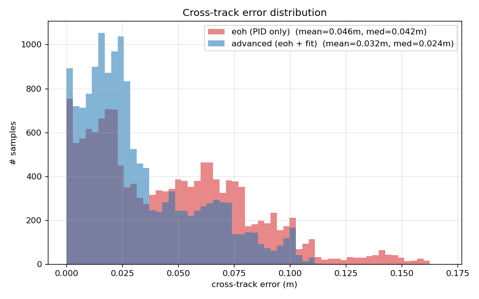
Distribution of cross-track error per odom sample. Advanced shifts the distribution toward zero.
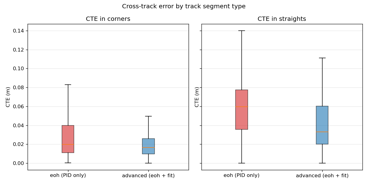
CTE split by corner and straight samples. Both improve; the straights improve more.
Speed & lap time
| metric | wall-balance (m/s) | advanced (m/s) | Δ |
|---|---|---|---|
| mean speed | 1.523 | 1.561 | +0.038 |
| mean in corners | 1.324 | 1.331 | +0.007 |
| mean in straights | 1.677 | 1.735 | +0.057 |
| min in corners | 0.843 | 0.991 | +0.148 |
| max | 1.996 | 2.000 | +0.003 |
| condition | lap 1 | lap 2 | lap 3 | lap time (mean ± std) | avg v |
|---|---|---|---|---|---|
| wall-balance | 14.95 s | 15.00 s | 15.01 s | 15.00 ± 0.03 s | 1.513 m/s |
| advanced | 14.60 s | 14.61 s | 14.56 s | 14.59 ± 0.03 s | 1.555 m/s |
Advanced is 0.4 s faster per lap (−2.7 %). Lap-to-lap variance is low in both conditions (std ≈ 30 ms).
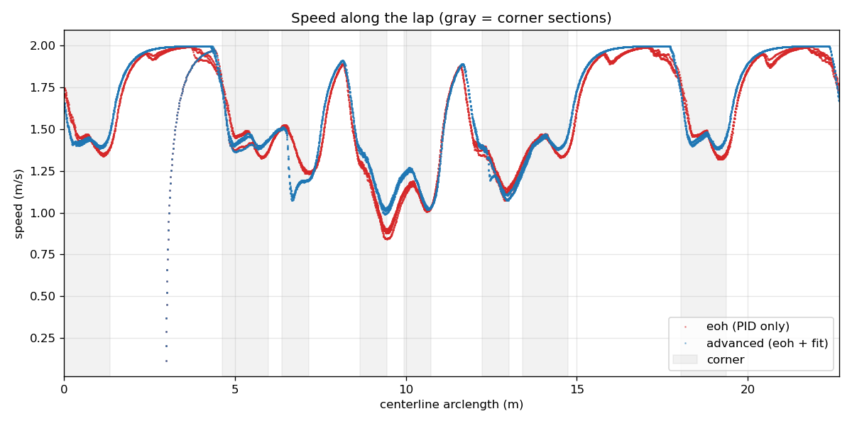
Speed trace over a lap’s arclength. Advanced holds the speed floor higher through the notch.
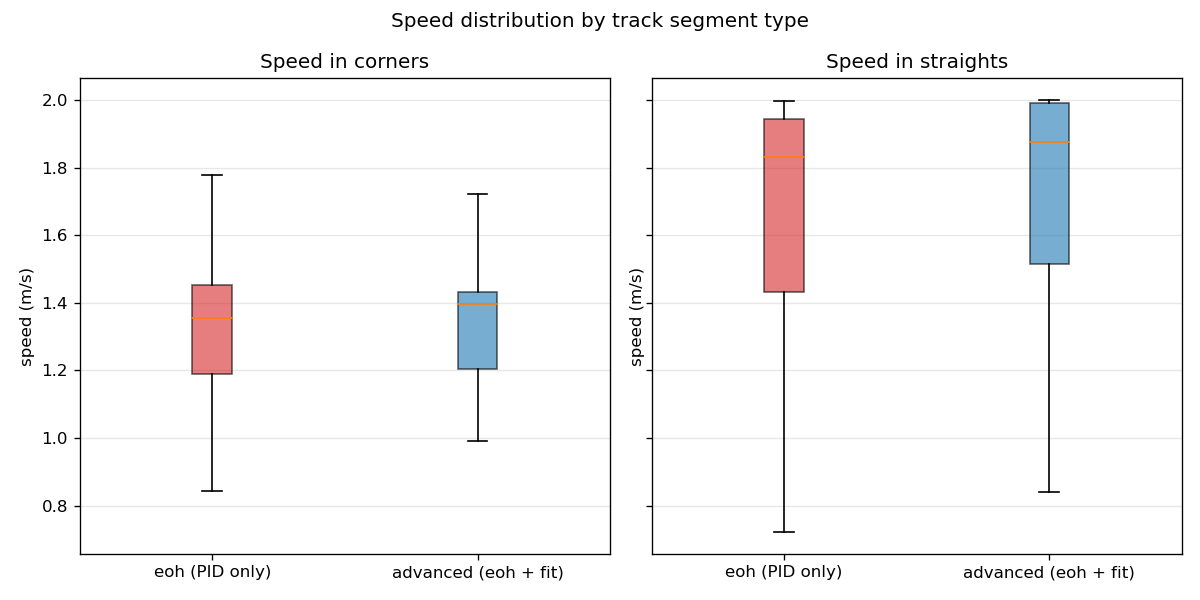
Mean speed in corner and straight segments.
Trajectories and per-lap velocity
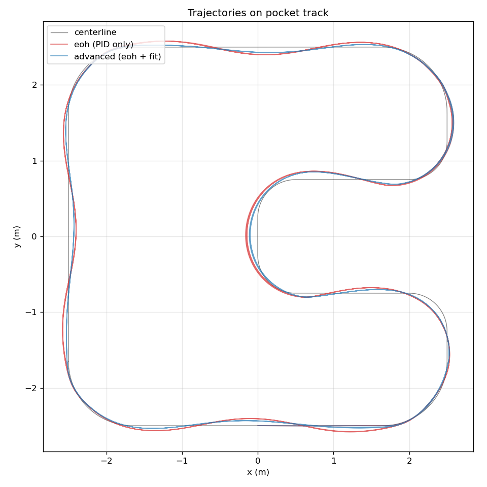
Driven trajectories overlaid on the centerline. The advanced path stays closer to the centerline on straights and cuts less into the notch-corner apices.
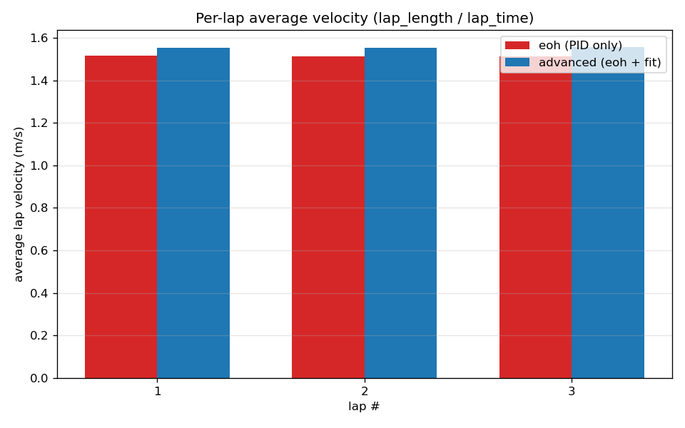
Per-lap average velocity across 3 full laps, each condition.
Observations
- Centerline tracking improves. Mean CTE drops by ~30 %, p95 by ~20 %. The bounded heading feedforward is the dominant contributor, and its effect is on straights rather than corners.
- The curvature speed cap is conservative. The notch radii are 0.5 m, which drives
v_curv ≈ √(a_lat / |κ|)toward 1 m/s. The Wall-Balance baseline cleared the same corners at ~1.3 m/s using forward-clearance speed alone. The cap accounts for most of the remaining corner-speed gap. Raisinglateral_accel_limitor relaxing the cap tomin(v_wb, α · v_curv)withα > 1would recover this. - No safety regression. Zero collisions in either condition. Lap-time variance is unchanged. The health-gated bounded design provides improvements when trusted and passthrough when not.
Parameters
- Max Speed: Upper speed limit for the car on the track, especially useful on the straights where the car doesn’t need to slow down to make turns.
- Max Steering Angle: Range for clipping the steering angle to avoid actuator saturation, can be adjusted to allow the car to make sharper turns (as long as it stays within actuator limits).
- Quadratic Residual Threshold: The maximum error our quadratic fit can have before we fall back to our distance-based driving code (error is calculated from comparing the fit and its predicted points to the real lidar point cloud).
- Quadratic Lookahead: The number of waypoints to look ahead for the pure pursuit controller to determine steering angle and speed.
- k_P, k_I, k_D (for steering): PID coefficients used for our fallback controller.
Milestone Status
ECE 484 measures F1Tenth teams against Milestone 2 (software) complete and Milestones 3–4 (hardware) in progress at the midpoint checkpoint.
Lessons Learned
Extend, do not replace. The pure-quadfit first pass was worse than the Wall-Balance baseline on the corners Wall-Balance was tuned for. Keeping Wall-Balance as an always-on inner loop and making the fit layer a bounded perturbation preserved smoother straights and corner-entry prediction without losing the safety floor.
Multi-frame gating matters more than sanity checks. Per-frame sanity (MAD reject, coefficient bounds) removed ~10 % of bad fits. The multi-frame gates (sign-of-b consistency, σ-of-b stability) removed the catastrophic cases: the corner-entry b-flips that caused crashes. The cost is a K-scan delay on the augmentation, 12 ms at 250 Hz, which does not affect control.
Define the metric before tuning. Early tuning was visual (“looks smoother”). Once study/analyze.py existed (CTE mean and p95, corner and straight split, per-lap time), tuning lateral_accel_limit and heading_gain took one evening rather than a week. The analysis also showed that the curvature cap was over-binding on the notch rather than simply slow.
Procedurally-generated maps catch issues early. The hairpin map exposed saturation of steering authority on tight U-turns. The snake map surfaced an alternation bug in wall assignment. The pocket map’s notch was designed so the curvature cap would bind. Each map took roughly 2 hours of Python to generate.
Final Words
Going with a simple approach worked best for our project, and our enhancements provided through the quadratic fit extension allowed our car to operate at an even higher speed than just the base code. The project was ultimately a great learning experience and we had a good time racing our car against the rest of the class, placing 3rd amongst all ECE 484 groups!
Team & Timeline
Arjun Chainani. Controls and integration. Wall-Balance PID implementation in ROS 2, quadratic fit and health-window design, parameter tuning across tracks.
Sam Lee. Simulation and analysis. Procedural map generation, comparison-study harness, analysis pipeline (CTE, speed, lap), site.
Suryansh Singh. Hardware and perception. CSL Studio bring-up, ROSBAG collection and annotation, camera-lane pipeline (post-midpoint).
| Week | Period | Milestone | Status |
|---|---|---|---|
| 1–2 | Jan 2026 | Research, architecture, simulator stand-up | ✅ Done |
| 3–4 | Jan–Feb 2026 | Wall-Balance PID + ROS 2 package scaffolding | ✅ Done |
| 5–6 | Feb–Mar 2026 | Procedural maps, quadfit prototype (failed pass) | ✅ Done |
| 7 | Mar 2026 | Health-gated advanced controller | ✅ Done |
| 8 | Apr 2026 | Cross-comparison study + writeup | ✅ Done (Apr 21) |
| 9–10 | Apr–May 2026 | Hardware deployment + on-car tuning | ✅ Done |
| 11–12 | May 2026 | Multi-track hardware robustness + final report | ✅ Done |
Reproduce
The repository is at github.com/arjunchainani/ece-484-f1tenth (branch lane-follower-dev).
# one-time environment setup (Ubuntu 22.04, see SETUP.md for detail)
./setup_f1tenth.sh
colcon build --symlink-install
source install/setup.bash

# run the autonomy stack against the sim
./run.sh all              # sim + lane_follower together

# reproduce the comparison study
study/run_comparison.sh 60
python3 study/analyze.py  # writes study/output/*.png + study/REPORT.md
Params are in src/lane_follower/config/lane_follower_params.yaml; toggle enable_advanced: true/false to switch layers. Sim track is selected in src/f1tenth_simulator/f1tenth_gym_ros/config/sim.yaml.
References
[1] O’Kelly, M., Sukhil, V., Abbas, H., Harkins, J., Kao, C., Pant, Y.V., Mangharam, R., Agarwal, D., Behl, M., Burgio, P., Bertogna, M. (2019). F1/10: An Open-Source Autonomous Cyber-Physical Platform. arXiv:1901.08567. [code]
[2] Coulter, R.C. (1992). Implementation of the Pure Pursuit Path Tracking Algorithm. Technical Report CMU-RI-TR-92-01, Carnegie Mellon University Robotics Institute. (Reference for the geometric steering law we use as a comparison baseline.)
[3] Snider, J.M. (2009). Automatic Steering Methods for Autonomous Automobile Path Tracking. Technical Report CMU-RI-TR-09-08, Carnegie Mellon University Robotics Institute.
[4] Sukhil, V. & Behl, M. (2021). Adaptive Lookahead Pure-Pursuit for Autonomous Racing. arXiv:2111.08873. (Context for the adaptive-lookahead approach we plan to layer on once hardware lane-following is stable.)
[5] Evans, B.D., Jordaan, H.W., Engelbrecht, H.A. (2024). Unifying F1Tenth Autonomous Racing: Survey, Methods and Benchmarks. arXiv:2402.18558. (Survey of the F1Tenth controller design space that motivated our bounded-combiner pattern.)
[6] Heilmeier, A., Wischnewski, A., Hermansdorfer, L., Betz, J., Lienkamp, M., Lohmann, B. (2020). Minimum Curvature Trajectory Planning and Control for an Autonomous Race Car. Vehicle System Dynamics 58(10). doi:10.1080/00423114.2019.1631455. (Source for the offline racing-line optimization in src/planning/, reserved for post-midpoint work.)
[7] Rousseeuw, P.J. & Croux, C. (1993). Alternatives to the Median Absolute Deviation. Journal of the American Statistical Association 88(424). (Basis for our MAD outlier reject in the wall fit.)
[8] Thrun, S., Burgard, W. & Fox, D. (2005). Probabilistic Robotics. MIT Press. Ch. 4: Nonparametric Filters. (Context for the particle-filter localization reserved for post-midpoint work.)
BibTeX
@techreport{tentenths2026midpoint,
  author      = {Chainani, Arjun and Lee, Sam and Singh, Suryansh},
  title       = {Ten Tenths: A Bounded-Augmentation LiDAR Autonomy Stack
                 for the F1Tenth Platform},
  institution = {University of Illinois Urbana-Champaign},
  year        = {2026},
  month       = {apr},
  note        = {ECE 484 Midpoint Checkpoint, Spring 2026},
  url         = {https://github.com/arjunchainani/ece-484-f1tenth}
}